Faster Geo Searches
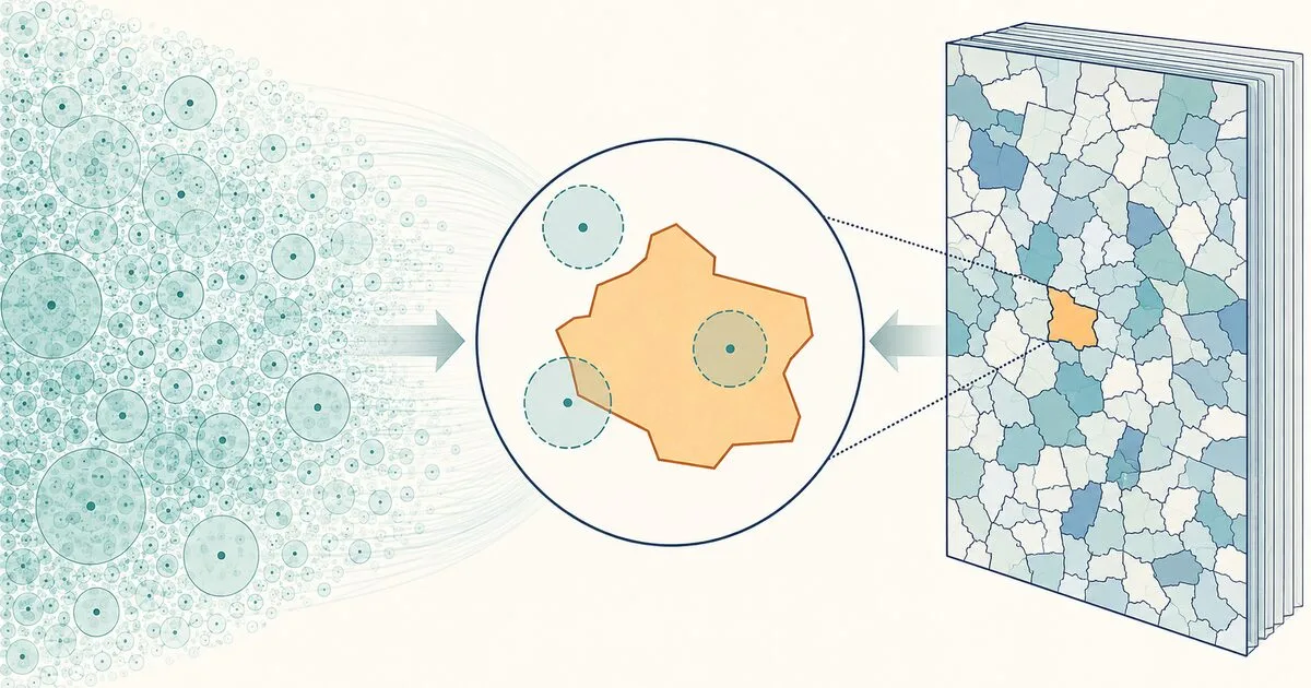
This paper presents the Tailored Geo-Query Scan, an algorithm specialized for billions of changing location-accuracy circles queried against a reusable family of neighborhood polygons.
Part I — The Specific Case
1. Billions of Circles Against 20,000 Neighborhoods
We need to test billions of changing location-accuracy circles against roughly 20,000 reusable neighborhood polygons
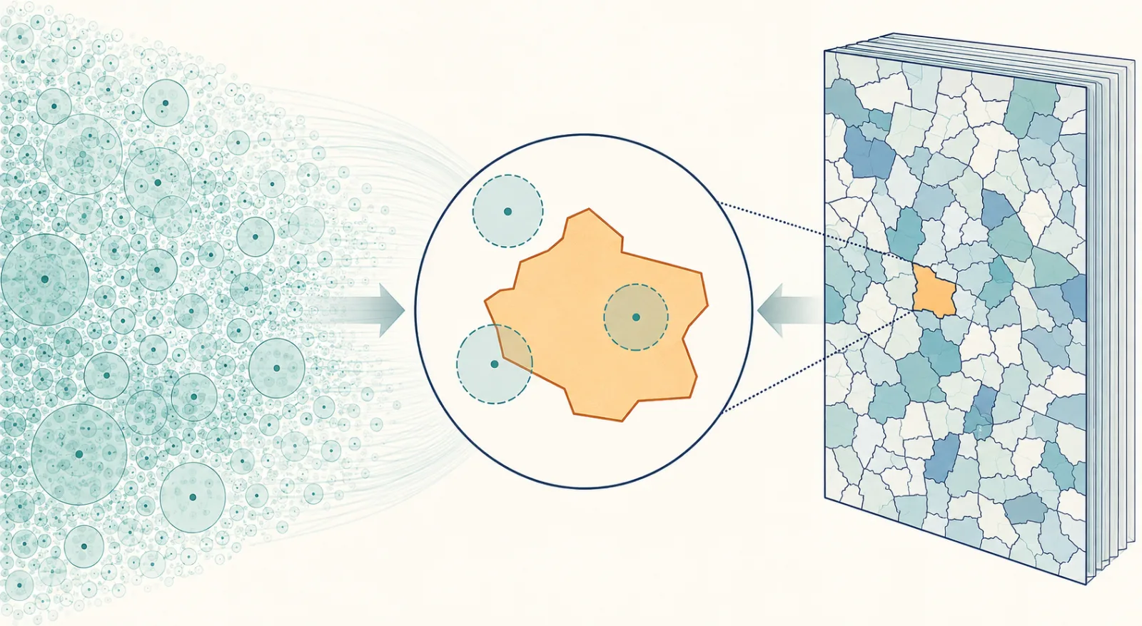
Each location is (x, y, radius), so a circle can intersect a neighborhood even when its center is outside. The goal is the fastest
exact intersection algorithm without expanding every circle into a larger spatial object.
Every query returns no more than 10,000 matching row IDs; it does not require an exact total, exhaustive aggregations, or a global sort.
We start with 10M to explain the algorithms and scale up to billions of circles and millions of queries.
2. The Naïve Exact Algorithm
For a circle with center c, radius r, and polygon P:
intersects(c, r, P)
    = center_inside(c, P)
      OR
      minimum_distance(c, polygon_edges(P)) <= r
Assume one query over 10 million circles and a representative neighborhood with roughly 300 edges.
The naïve algorithm first tests the center against every edge. For centers outside the polygon—and most centers are outside one particular neighborhood—it then calculates the distance to every edge.
center-inside work     10M circles × 300 edges  = 3B edge calculations
edge-distance work    ~10M circles × 300 edges  = 3B edge calculations
                                                       ───
naïve query                                         ≈ 6B edge calculations
The mathematics is simple. Performing it about six billion times for every neighborhood query is the problem.
Part II — Comparing Algorithms: Metrics and Results Summary
3. Elasticsearch Indexing Versus Scanning
10M Benchmark Metrics and Results
For the same 10 million circles, we compare Elasticsearch's triangle index with the naïve exact scan and the Tailored Geo-Query Scan. We evaluate each plan by its geometry work, hot geometry size, and hot query time:
- Geometry work — how many edge or triangle units we create or evaluate.
- Hot geometry size — how much data must remain in memory or the operating-system page cache.
- Hot query time — the observed scale after caches are warm.
The values below are deliberately rounded. They normalize the current Ramat Gan experiment to 10 million circles so the order of magnitude remains visible.
| Plan | Dominant geometry work for 10M circles | Hot geometry size | Hot query scale |
|---|---|---|---|
| Naïve exact | ≈6B edge calculations | ≈120 MB | ≈2 s |
| Elasticsearch triangles at 15 m | ≈130M indexed triangles | ≈4 GB | ≈1.2 s |
| Tailored Geo-Query Scan | ≤10M fast checks; up to ≈300M fallback edge calculations | ≈124 MB | ≈0.2 s |
These times describe one hot query on the benchmark machine, not a universal service guarantee. The important result is the scale: the triangle index trades storage for tree pruning, while the Tailored Geo-Query Scan removes most expensive geometry work before it starts.
Scaling Metrics and Results
At production scale, we compare both algorithms across 10B or 100B circle rows and 1M or 10M queries per day using peak query rate, required cluster size, and monthly infrastructure cost.
The estimates concentrate daily traffic into ten working hours, giving 27.8 or 277.8 queries per second. Every query returns at most 10,000 row IDs and has a 95th-percentile latency target below one second. Elasticsearch includes one-node failure headroom; the Tailored Geo-Query Scan starts replacement workers from a shared filesystem instead of paying for an idle hot spare.
| Rows | Queries/day | Peak QPS | ES cluster | ES/month | Tailored cluster | Tailored/month |
|---|---|---|---|---|---|---|
| 10B | 1M | 27.8 | 3D+5S | $7.7K | 1W + FS | $2.9K |
| 10B | 10M | 277.8 | 16D+5S | $36.4K | 1W + FS | $2.9K |
| 100B | 1M | 27.8 | 16D+5S | $37.2K | 1W + FS | $6.7K |
| 100B | 10M | 277.8 | 150D+5S | $332.7K | 1W + FS | $6.7K |
D and W mean one AWS i7i.8xlarge: 32 vCPUs, 256 GiB RAM, and 7.5 TB local NVMe. S means three
m7i.xlarge masters and two m7i.2xlarge coordinators. FS means shared FSx for Lustre storage.
These are capacity estimates, not benchmark results for the proposed clusters. Parts III–V explain the algorithms and derive the resource estimates behind this summary.
Part III — How Elasticsearch's Triangle Index Works
4. Add a Triangle Index
Elasticsearch cannot index a circle directly as an exact circle. Its circle ingest processor approximates each circle with a regular polygon, tessellates that polygon, and stores the triangles in a Lucene BKD tree.
circle
    ↓ approximate with polygon
about 15 vertices
    ↓ tessellate
about 13 triangles
    ↓ index
BKD tree
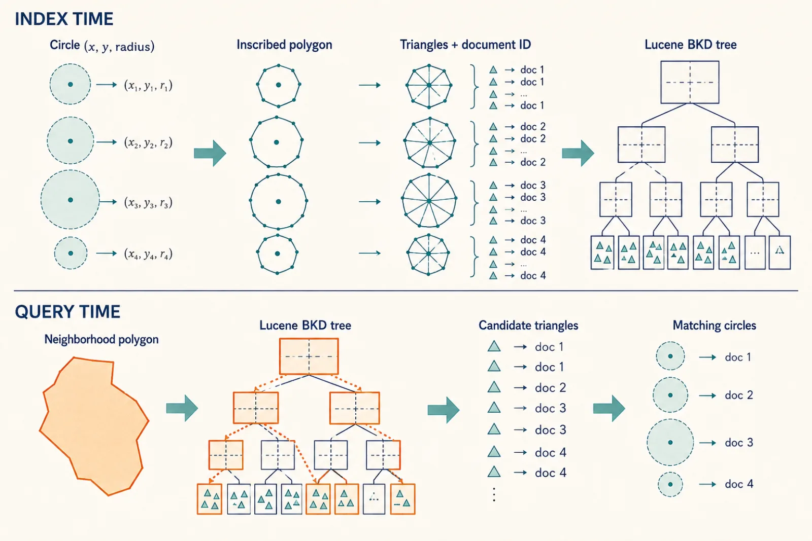
With the benchmark's 15 m approximation error, one circle produces about 13 triangles on average:
10M circles × about 13 triangles ≈ 130M indexed triangles
Resolution Is a First-Order Cost
Elasticsearch calls this setting error_distance. It is not a map-grid resolution: it is the permitted inward gap between the true
circle radius and a side of the inscribed polygon. A smaller gap requires more polygon sides, and every additional side creates another
triangle for almost every one of the 10 million circles.
The rounded triangle counts use the benchmark's real 15–350 m radius distribution. The 15 m and 100 m index sizes are measured; the 1 m and 1 km sizes are estimates based on those two real values.
| Error distance | Average sides per circle | Triangles for 10M circles | Primary index size |
|---|---|---|---|
| 1 m | ≈58 | ≈560M | ≈11 GB |
| 15 m | ≈15 | ≈130M | ≈4 GB |
| 100 m | ≈6 | ≈40M | ≈2.5 GB |
| 1 km | 4 | 20M | ≈2 GB |
Moving from 1 m to 1 km reduces the triangle count by roughly 28×, but the index by only about 5× because Lucene still keeps document and tree overhead. At 1 km every circle reaches Elasticsearch's minimum four-sided polygon because every radius is at most 350 m.
The performance gain is purchased with lost geometry. The polygon is inside the true circle, so coarse settings can miss real intersections near the circular boundary. In the measured runs, moving from 15 m to 100 m reduced the hot-query scale from roughly 1.2 seconds to 0.6 seconds, while increasing the number of missed exact matches.
How a Query Uses the Index
Each Elasticsearch shard is a Lucene index made of immutable segments. Every segment has its own BKD tree and segment-local document IDs, so a query runs separately against every relevant segment.
The BKD tree compares the neighborhood with spatial cells, skips branches that cannot intersect it, and descends through overlapping cells to candidate triangles. Lucene maps matching triangles back to document IDs, combines them with the other query clauses, and Elasticsearch merges the results from all shards.
Other clauses may use document-ID iterators or cached bitsets; they do not necessarily produce one universal bitmap. The explicit input and output bitmaps in Section 8 belong to the Tailored Geo-Query Scan plugin integration.
Part IV — How the Tailored Geo-Query Scan Works
5. Fast Scan, Exact Scan When Needed
The Tailored Geo-Query Scan leaves every circle as three float32 values:
x, y, radius = 12 bytes
10M circles × 12 bytes = 120 MB
Its fast scan produces one of three outcomes:
NO       bounding boxes prove no intersection
YES      a certified inner shape proves intersection → append row ID
MAYBE    save for the exact scan, if needed
Every YES is a final exact match. The fast scan stops and returns as soon as it collects 10,000 YES row IDs; in that case, the exact
scan never runs. Only if the fast scan ends below 10,000 does the exact scan evaluate MAYBE circles, stopping at 10,000 total matches
or when no MAYBE circles remain.
Without early termination, the Ramat Gan distribution rounds cleanly at 10 million circles:
10M circles
    ├─ about 9M bbox NO
    └─ about 1M bbox survivors
           ├─ about 0.5M fast YES
           └─ about 0.5M MAYBE → exact geometry
Only the half-million MAYBE circles pay for the polygon edges. Two 300-edge passes produce roughly 300 million heavy edge
calculations, about twenty times fewer than the naïve six-billion calculation path. This is the full fallback path; a query that
reaches 10,000 YES results during the fast scan pays none of this exact-geometry work.
The hot working set is approximately:
circle buffer                      120 MB
input, output, and MAYBE bitmaps    about 4 MB
compiled neighborhood               about 10 KB
That is roughly 124 MB, small enough to keep hot on an ordinary server. The measured native and plugin results scale to roughly 0.2 seconds for 10 million circles.
6. Compile the Reused Neighborhood
The circles arrive continuously; the 20,000 neighborhood polygons change rarely. We therefore compile polygons rather than expanding every circle.
The GeoScan Image
For each neighborhood, the GeoScan Image stores:
polygon bounding box
prepared edge records
certified inner rectangles
geometry hash, offsets, counts, and checksum
Ramat Gan has roughly 300 edges and compiles to roughly 10 KB. The GSI file is memory-mapped, and a canonical hash of the query vertices selects the compiled polygon without parsing or allocation in the hot path.
Bounding Boxes Prove NO
The outer bounding box is a conservative NO proof:
circle does not overlap polygon bounding box → NO
Inner Rectangles Prove YES
The compiler also finds large rectangles completely contained by the polygon. They are conservative YES proofs:
inner rectangle ⊆ polygon
circle intersects inner rectangle
therefore circle intersects polygon → YES
Neither proof changes the answer. An inconclusive result becomes MAYBE, never an incorrect YES or NO.
MAYBE Continues to the Exact Scan
For each MAYBE, the exact stage checks whether the center is inside the polygon and, if not, measures the center against polygon
edges. Squared distances avoid square roots.
7. Shape the Data for SIMD
Sixteen circles are stored as one AVX-512 structure-of-arrays block:
[x0  x1  ... x15]
[y0  y1  ... y15]
[r0  r1  ... r15]
The CPU loads sixteen centers and radii, performs the same bounding-box comparisons on all lanes, and returns a 16-bit survivor mask. Ten million circles require only 625,000 vector blocks for the fast scan.
The point is not that every instruction becomes sixteen times faster. The point is that the common path is contiguous data, vector comparisons, and masks rather than objects, branches, and per-row calls.
8. Exchange Segment-Local Bitmaps
The Tailored Geo-Query Scan plugin runs once per Lucene segment. It materializes the documents selected by normal filters as a segment-local candidate bitmap:
tenant AND time AND other filters
                 ↓
         input segment bitmap
                 ↓
       Tailored Geo-Query Scan
                 ↓
        output segment bitmap
                 ↓
   aggregation, sorting, pagination
Bit N and circle-buffer position N both mean segment document ID N. A zero bitmap word skips 64 documents, and JNI crosses the
Java/native boundary once per segment rather than once per document.
The circle buffer and bitmaps are direct or memory-mapped buffers. Native code reads the same bytes as Java, so the query creates no second circle buffer and performs no circle-data copy.
Part V — Scaling Up
9. Four Production Cases
The Part II summary presents the four production outcomes. This part derives their storage, search-capacity, and cost estimates.
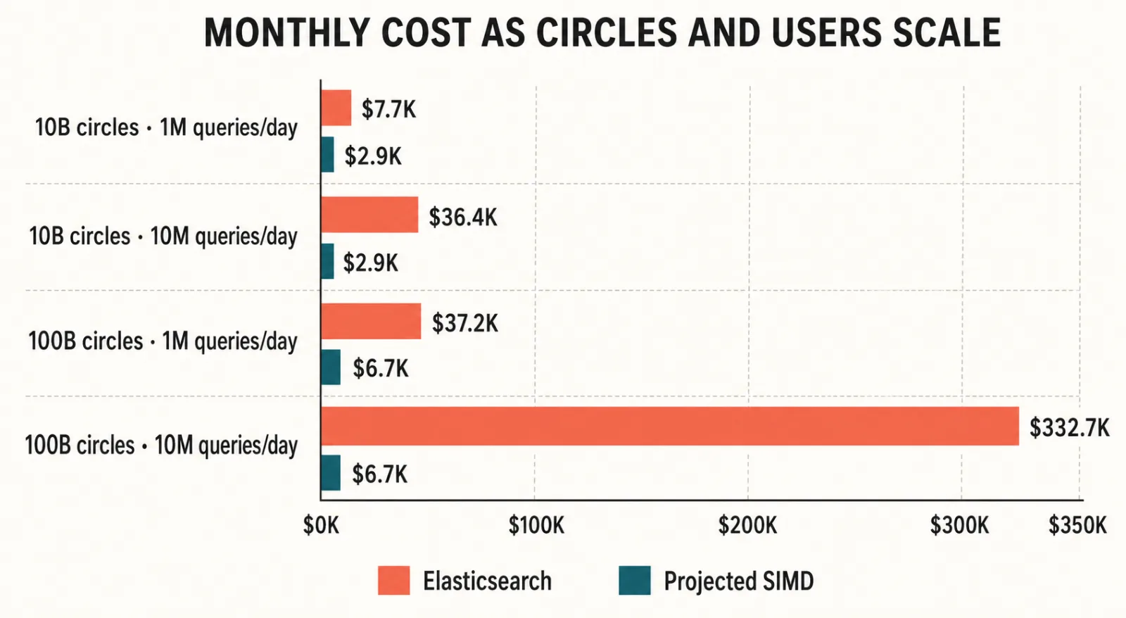
The cost bars show the outcome. The architectural picture shows why: Elasticsearch expands every stored circle into indexed triangles and grows its server fleet, while the Tailored Geo-Query Scan grows its storage but keeps emitting the same 10M-row query unit.
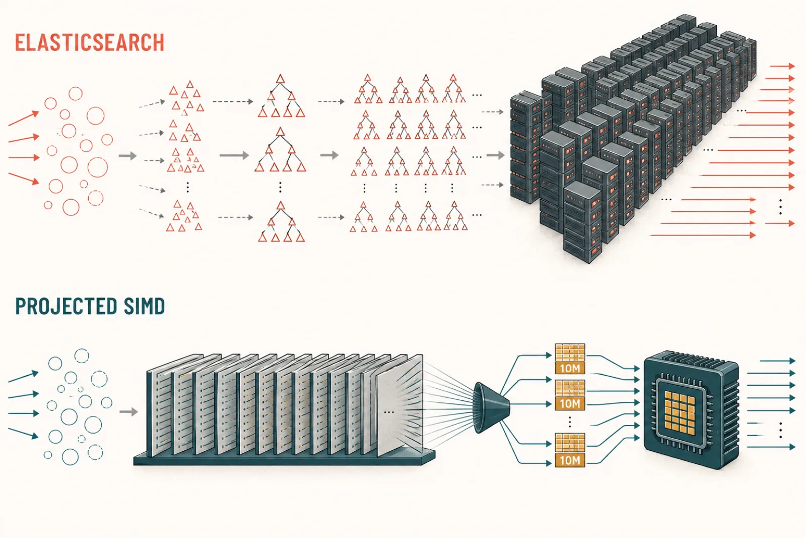
Monthly totals use Linux on-demand prices in us-east-1 for 730 hours and include one durable S3 copy. Local NVMe is included in the
instance price. Elastic licensing, Kubernetes control-plane fees, logging, network transfer, tax, and temporary ETL capacity are not
included.
These are capacity estimates, not benchmark results for the proposed cloud clusters. Their purpose is to expose the dominant resource in each design: Elasticsearch consumes search CPU and triangle-index storage; the Tailored Geo-Query Scan consumes memory and Parquet bandwidth.
10. Scaling Up with Elasticsearch
Storage Is Paid Before the First Query
At 15 m approximation error, the measured data produces about 13 indexed triangles per circle and a 4 GB primary index per 10M circles. Linear extrapolation gives:
| Rows | Indexed triangles | Primary geo index | Primary + one replica |
|---|---|---|---|
| 10B | ≈130B | ≈4 TB | ≈8 TB |
| 100B | ≈1.3T | ≈40 TB | ≈80 TB |
This excludes ordinary-field indexes and merge headroom. The 10,000-result limit does not reduce this ingest or storage cost because every circle is expanded and indexed before Elasticsearch knows which queries will arrive.
Using 50 GB primary shards gives roughly 80 primaries for 10B rows or 800 for 100B rows, plus their replicas. Those sizes also keep each shard below about 125M documents. Elasticsearch recommends 10–50 GB shards, fewer than 200M documents per shard, and warns that each shard executes a search on one CPU thread.
Search CPU Determines the Cluster
We assume routing and normal predicates reduce each query to 1/1,000 of the rows:
| Rows | Relevant rows/query | Measured-scale search work/query |
|---|---|---|
| 10B | 10M | ≈1.2 core-seconds |
| 100B | 100M | ≈12 core-seconds |
The second column is the selected logical data, not the whole index. The third linearly extrapolates the measured 15 m Elasticsearch query. We provision one effective search thread per vCPU and divide by 70% target utilization:
required vCPUs = peak QPS × core-seconds per query ÷ 0.70
| Rows | Queries/day | Search vCPUs | Data nodes for capacity | Data nodes with N+1 |
|---|---|---|---|---|
| 10B | 1M | ≈48 | 2 | 3 |
| 10B | 10M | ≈476 | 15 | 16 |
| 100B | 1M | ≈476 | 15 | 16 |
| 100B | 10M | ≈4,762 | 149 | 150 |
The 100B/1M cluster also matches the storage floor: sixteen data nodes provide 120 TB of raw local NVMe for the estimated 80 TB index with replicas and operating headroom. At higher traffic, CPU—not disk capacity—sets the node count.
A single shard thread would take about 1.2 seconds for 10M relevant rows or 12 seconds for 100M. To leave 0.7 seconds of the SLA for search, a query must spread across at least two or eighteen shard tasks respectively. Routing must therefore narrow the search without collapsing all selected rows onto one shard.
Elasticsearch's size: 10000 limits the response, not necessarily the evaluated documents. terminate_after is per shard and applies
before sorting. Early termination may improve these estimates, but it must be measured; it cannot be used to erase the indexed
triangles or assumed to stop all shards at one global 10,000-hit counter.
Elasticsearch Cost
An i7i.8xlarge is $3.0202/hour, or about $2,205/month. The five support nodes add about $1,030/month. One S3 copy of the primary geo
index adds about $92/month at 10B rows or $920/month at 100B rows. This produces the Elasticsearch totals in the opening chart.
11. Scaling Up with the Tailored Geo-Query Scan
Prepare for Known Query Patterns
The Tailored Geo-Query Scan does not maintain a triangle index. It builds two Parquet projections ordered for the two known predicate patterns and divides them into 10M-row query slices. A query chooses one projection, uses partition and row-group metadata to locate one slice, and never scans the other projection.
query pattern → projection → partition → Parquet row groups
                                             ↓
                                  dense 1M-circle buffer
                                             ↓
                                  Tailored Geo-Query Scan
                                             ↓
                                     first 10K row IDs
One logical projection row contains two 32-bit properties, three float32 circle values, and a 64-bit row ID: 28 bytes. Two projections therefore contain about 560 GB for 10B rows or 5.6 TB for 100B rows before Parquet compression. The query reads only the columns and partition it needs.
One Query Has a Small Working Set
| Rows | Property rows/query | Two-property payload | Dense circle buffer | Modeled query time |
|---|---|---|---|---|
| 10B | 10M | 80 MB | ≈20 MB | ≈38 ms |
| 100B | 10M | 80 MB | ≈20 MB | ≈38 ms |
The dense buffer holds one million circles: 12 MB of x/y/radius, 8 MB of row IDs, and a small result bitmap. Its exact geometry scan
takes approximately 30 ms under the conservative 0.3 seconds per 10M-circle assumption. We assume the first buffer produces at least
10,000 matches with very high probability.
If it does not, the engine resumes the same Parquet slice and reuses the 20 MB workspace. It processes up to 100 MB of circle payload, about 8.3M circles and 0.25 seconds of geometry. It stops at 10,000 matches, at the end of the selected slice, or at the 100 MB safety limit. Reaching the limit without 10,000 matches returns an explicit error rather than a partial result.
Query Rate Determines the Worker Count
The capacity model counts the property bytes plus the compacted candidate buffer:
| Rows | Queries/day | Aggregate decoded traffic | Active workers |
|---|---|---|---|
| 10B | 1M | ≈2.8 GB/s | 1 × i7i.8xlarge |
| 10B | 10M | ≈27.8 GB/s | 1 × i7i.8xlarge |
| 100B | 1M | ≈2.8 GB/s | 1 × i7i.8xlarge |
| 100B | 10M | ≈27.8 GB/s | 1 × i7i.8xlarge |
The total dataset does not enter the online calculation after the projection directory resolves the 10M-row slice. Both sizes produce the same 80 MB property scan, 20 MB dense circle buffer, and query rate. One 32-vCPU worker therefore serves every modeled case; the 100B design differs only in disk capacity. Sustaining the assumed extraction rate remains a required production benchmark.
Shared Storage Replaces the Hot Backup
The immutable projection generation lives on FSx for Lustre and has one durable copy in S3. A replacement worker mounts the same filesystem, accepts degraded work immediately, and copies only its assigned partitions to local NVMe or RAM. No idle compute replica runs permanently.
We price Persistent 2 SSD at the 1,000 MB/s/TiB tier: $0.60/GB-month in us-east-1. The 10B case uses the 1.2 TB minimum, costing
$720/month and delivering 1.2 GB/s baseline throughput. The 100B case uses 7.2 TB, costing $4,320/month. S3 adds about $13 or $129.
| Rows | Active compute | Shared FS | Durable S3 | Total/month |
|---|---|---|---|---|
| 10B, either traffic level | 1 × $2,205 | $720 | $13 | $2.9K |
| 100B, either traffic level | 1 × $2,205 | $4,320 | $129 | $6.7K |
Mounting is fast; warming is not instant. At 1.2 GB/s, loading the 160 GB 10B predicate set has a 133-second transfer floor, while reading the full 560 GB generation takes 7.8 minutes. The 100B generation is ten times larger, but a worker can serve selected slices directly from the mounted filesystem while its local cache warms. Recovery time is a production benchmark, not a boot-time promise.
Assumptions
- Projection and row-group pruning must consistently resolve each query to its intended 10M-row slice.
- The first one-million-circle batch must produce 10,000 matches at the expected probability; fallback frequency must remain low. or the query can fail
Part VI — Conclusion
12. Why the Tailored Geo-Query Scan Fits This Case
For arbitrary changing shapes and many spatial relations, Elasticsearch's triangle index remains the general solution. For billions of compact circles queried against a reused library of neighborhoods, the Tailored Geo-Query Scan is the most effective algorithm: reject by bounding box, accept by certified inner shapes, and run exact edge geometry only for the unresolved circles.
References
Elasticsearch — Circle processor
https://www.elastic.co/guide/en/elasticsearch/reference/current/ingest-circle-processor.htmlElasticsearch — geo_shape field type
https://www.elastic.co/docs/reference/elasticsearch/mapping-reference/geo-shapeElastic — BKD-backed geo_shapes
https://www.elastic.co/blog/bkd-backed-geo-shapes-in-elasticsearch-precision-efficiency-speedElastic — Tune for search speed
https://www.elastic.co/guide/en/elasticsearch/reference/current/tune-for-search-speed.htmlElasticsearch — Size your shards
https://www.elastic.co/docs/deploy-manage/production-guidance/optimize-performance/size-shardsElasticsearch — Search API and per-shard
terminate_afterhttps://www.elastic.co/guide/en/elasticsearch/reference/current/search-search.htmlElasticsearch — Paginate search results and
sizehttps://www.elastic.co/docs/reference/elasticsearch/rest-apis/paginate-search-resultsElasticsearch — Boolean filter clauses
https://www.elastic.co/docs/reference/query-languages/query-dsl/query-dsl-bool-queryElasticsearch — Node query cache
https://www.elastic.co/guide/en/elasticsearch/reference/8.19/query-cache.htmlAWS — EC2 I7i specifications
https://aws.amazon.com/ec2/instance-types/i7i/AWS — EC2 on-demand pricing
https://aws.amazon.com/ec2/pricing/on-demand/AWS — S3 pricing
https://aws.amazon.com/s3/pricing/Current
i7i.8xlargepublic price listinghttps://cloudprice.net/aws/ec2/instances/i7i.8xlargeCurrent
m7i.2xlargepublic price listinghttps://cloudparity.io/pricing/aws/m7i.2xlarge?os=linux&price_model=ondemand®ion=us-east-1AWS — FSx for Lustre pricing
https://aws.amazon.com/fsx/lustre/pricing/AWS — FSx for Lustre and S3 data repositories
https://docs.aws.amazon.com/fsx/latest/LustreGuide/fsx-data-repositories.html